(*) 第六節 - FFT 的應用三（大規模的線性摺積）

# 問題的動機

有時我們在處理訊號的時候往往會遇到非常巨量的資料，倘若此時還堅持使用上一節的方法，根據本文件的參考課本 [7] 第 394 頁右下角所述，基於以下三大理由，會變得非常不方便。

輸入訊號的長度可能不是個定值。
輸入訊號的長度可能太長。
輸出訊號的計算必須等到輸入訊號全數收集完畢後才能進行。

有鑑於此，我們在本節會介紹一些分段消化的技巧，簡單來說就是每一小段的輸入訊號都和濾波器作線性摺積之後再拼起來，而這個摺積其實未必要用 FFT 實作，土法煉鋼的方式也可以，只是誠如第三節所說，在資料量大的時候都用 FFT 取代 DFT 只有好處沒有壞處。閱讀的時候，請盡量把注意力放在圖片上，因為程式碼繁雜可能不易理解，一旦理解圖片所呈現的架構，自然可以自己實作出來。

這一節是選讀章節，因為實際上在寫作業的時候不太會遇到巨量資料的情況，故除非以後有要往比較專精的領域發展，不然對初學者來說其實不用急於理解這邊所提的兩個方法。

# 方法一 (重疊-相加法、overlap-add method)

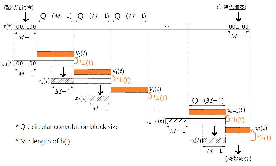
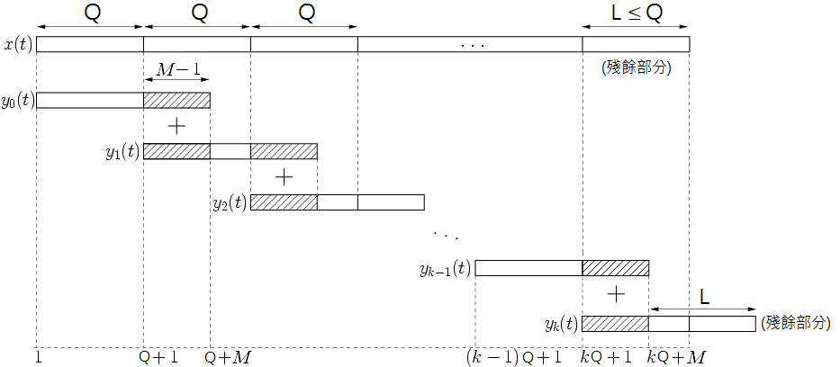
簡單來說，就是把輸入訊號切成很多連續緊鄰的小區間，依此跟濾波器作摺積，只不過這樣子做會有一個小問題，以下面這張示意圖來說，每個 $y_i$ 都是 $x_i*h$ ，但是我們稍微想一下就知道，其實後半段的輸出 $y_i(Q+1)$ 到 $y_i(Q+M-1)$ 都是不完整的，因為這個階段的輸出沒有考慮到下一階段的輸入 $x_{i+1}$ ，輸入是連續的，理論上後半段的輸出也要同時從接下來的輸入計算出來才行，因此這部分必須再加上下面一個區間的前半段之計算結果，才會完備。

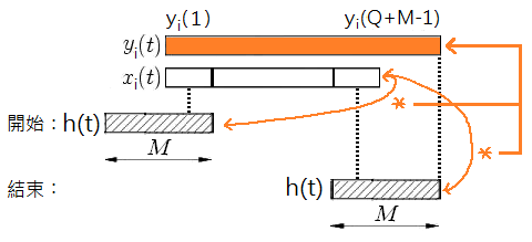
每個 $y_i$ 的產生方式

演算法架構 (僅列出 $x_i$ 和 $y_i$ 的關係，沒有列出 $h$ )

MATLAB 呈現 (現實版：只要訊號源長度滿一個區塊單位就開始即時運算)

function y = overlap_add(h,x,Q) % Q: one input block length
    y = []; % declare output signal array
    M = length(h); % M: filter length
    buf = zeros(1,Q+M-1); % buffer: 上圖的 y_i(t)
    m = 0; % index of the block number
    while (m+1)*Q < length(x) % if the current input block is not the last one
        buf = buf + conv(h, x(m*Q+(1:Q))); % perform convolution of one block and add to the buffer
        buf(1:Q) % print one block of signal
        y = [y,buf(1:Q)]; % append the printed block to the final result
        buf(1:M-1) = buf(Q+1:end); % left-shift the buffer by one block length. i.e., move the non-complete part of length M-1 to the front
        buf(M:end) = 0; % the remaining vacant parts should be initialized to zero
        m = m + 1; % go to the next block
    end
    tmp = conv(h, x(m*Q+1:end)); % perform convolution on the last block
    buf = buf(1:length(tmp)) + tmp % add to the buffer and print it
    y = [y,buf]; % append the last block to the result
end

MATLAB 呈現 (簡化版：等到訊號源輸入完畢才開始運算)

function y=overlap_add(h,x,Q) % Q: one input block length
    L=length(x); M=length(h);
    Nblocks=ceil(L/Q);
    ni=(1:Q); no=(1:M+Q-1);
    y=zeros(1,L+M-1);

    for m=0:Nblocks-2
        z=conv(h,x(m*Q+ni));
        y(m*Q+no)= y(m*Q+no)+z;
    end

    z=conv(h,x((Nblocks-1)*Q+1:end));
    y((Nblocks-1)*Q+1:end)= y((Nblocks-1)*Q+1:end)+z;
end

計算實例

純數學運算 $\displaystyle \{x_n\} = 1,2,3,4,5,6,7,8,9,10,11,12,13,14,15,16,17,18,19,20$ $\displaystyle \{y_n\} = 10,20,30$ $\displaystyle \{x_n*y_n\}\ = 10,40,100,160,220,280,340,400,460,520,580,640,700,760,820,880,\\940,1000,1060,1120,970,600$

程式碼驗證

h = [10,20,30];
x = (1:20);
Q = 7;
overlap_add(h,x,Q) % Q can be replaced with any positive integer.
% ans = 10 40 100 160 220 280 340 400 460 520 580 640 700 760 820 880 940 1000 1060 1120 970 600

# 方法二 (重疊-儲存法、overlap-save method) [8]

相較於重疊-相加法，這邊我們拉長一個區間的長度，並且令區間與區間之間重疊，如此一來每個輸出區間便能獨自完成。魚與熊掌不可兼得，因為重疊的緣故，也會花上較多時間計算。

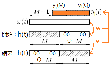
演算法之前的引理 (lemma)

當 $h$ 只補齊 $Q-M$ 個零，要和 $x_i$ 作循環摺積的時候，必須讓 $h$ 完全埋沒在 $x_i$ 的範圍裡面，因為唯有這個條件滿足時其他沒被覆蓋到的地方才會自動補零、而不影響線性摺積的結果，還沒全部進入摺積區的時候循環補零的長度有限，剩下的時點便會直接拿 $h$ 的訊號填充、進而影響線性摺積結果。不管補零的長度 $Q-M$ ( $x_i$ 的長度 $Q$ ) 有多長、甚至完全不補零 ( $Q=M$ )，這個引理都會成立，但是要記得務必維持 $Q\ge M$ 。下面的演算法便是依據這個引理的巧思設計而來。

演算法架構

我們會發現上圖每次都會輸出 $Q-M+1$ 個單位的訊號，大部分的參考資料都會直接給這個值一個名字以簡化敘述，但是這邊為了要減少符號的數量，就不給名字了，希望讀者直接把 $Q-M+1$ 記憶起來、當成每次前進的量。

MATLAB 呈現 (現實版：只要訊號源長度滿一個區塊單位就開始即時運算)

function y = overlap_save(h,x,Q) % Q: one circular convolution block length
    M = length(h); % M: filter length
    x = [zeros(1,M-1),x,zeros(1,M-1)]; % padding (M-1)-zeros to both sides of the input signal
    L = length(x); % L: input length
    if ~(Q>=M) % check validity of Q
        error('Q cannot be smaller than the filter length!');
    end

    y = [];
    h_pad = [h,zeros(1,Q-M)]; % zero padding h to the block length
    m = 0; % index of the block number
    while Q+m*(Q-M+1) < L % if the current block does not touch or exceed the boundary
        buf = ifft(fft(h_pad).*fft(x(m*(Q-M+1)+(1:Q)))); % perform circular convolution of one block
        buf(M:end) % print the valid part (i.e. not affected by circular convolution)
        y = [y,buf(M:end)]; % append the printed block to the final result
        m = m + 1; % go to the next block
    end

    h_pad = h_pad(1:length(h_pad)-(Q+m*(Q-M+1)-L)); % shrink padded h to the last block length
    buf = ifft(fft(h_pad).*fft(x(m*(Q-M+1)+1:end))); % perform circular convolution on the last block
    buf = buf(M:end) % print the valid part (i.e. not affected by circular convolution)
    y = [y,buf]; % append the last block to the result
end

MATLAB 呈現 (簡化版：等到訊號源輸入完畢才開始運算)

function y=overlap_save(h,x,Q) % Q: one circular convolution block length
    L=length(x); M=length(h);
    if ~(L>=Q && Q>=M) % check validity of Q
        error('Q must satisfy L>=Q && Q>=M.');
    end
    P=Q-M+1; % Overlap
    Nblocks=ceil((L-Q)/P+1);
    y=zeros(1,L+M-1);
 
    z=conv(x(1:Q),h);
    y(1:Q)=z(1:Q);
 
    for m=1:Nblocks-2
        z=cconv(h,x(m*P+(1:Q)),Q);
        y(Q+(m-1)*P+(1:P))= z(M:Q);
    end

    m=Nblocks-1;
    z=conv(h,x(m*P+1:end));
    y(Q+(m-1)*P+1:end)=z(M:end);
end

這邊簡化版的程式碼對頭尾區塊的處理不像現實版的實作方式是先補零再作循環摺積，而是不補零、直接作線性摺積，其實兩種作法都可，這邊採用後者純粹是為了方便。另一個差別就是現實版的程式碼是隨著演算法架構的示意圖，每次都輸出 $Q-M+1$ 個單位的訊號；簡化版程式碼則是先輸出一次 $Q$ 個單位的訊號，之後再每次輸出 $Q-M+1$ 個單位的訊號。

計算實例

純數學運算 $\displaystyle \{x_n\} = 1,2,3,4,5,6,7,8,9,10,11,12,13,14,15,16,17,18,19,20$ $\displaystyle \{y_n\} = 10,20,30$ $\displaystyle \{x_n*y_n\}\ = 10,40,100,160,220,280,340,400,460,520,580,640,700,760,820,880,\\940,1000,1060,1120,970,600$

程式碼驗證

h = [10,20,30];
x = (1:20);
Q = 7;
overlap_save(h,x,Q) % Q can be any positive integer larger than or equal to length(h).
% ans = 10 40 100 160 220 280 340 400 460 520 580 640 700 760 820 880 940 1000 1060 1120 970 600